
This page provides details on the design and analysis of bolted joints. This source of this page is Brown et al., "Guideline for Bolted Joint Design and Analysis: Version 1.0," Sandia Report SAND2008-0371, Sandia National Laboratories, 2008.
This document provides general guidance for the design and analysis of bolted joint connections. An overview of the current methods used to analyze bolted joint connections is given. Several methods for the design and analysis of bolted joint connections are presented. Guidance is provided for general bolted joint design, computation of preload uncertainty and preload loss, and the calculation of the bolted joint factor of safety. Axial loads, shear loads, thermal loads, and thread tear out are used in factor of safety calculations. Additionally, limited guidance is provided for fatigue considerations.
The purpose of this report is to document the current state of the art in bolted joint design and analysis and to provide guidance to engineers designing and analyzing bolted connections. There is no one right answer or way to approach all the cases. In many cases, additional work will be needed to assess the quality of current practices and provide guidance. General information, suggestions, and guidelines are provided here but ultimately the engineer must use his/her judgment on which approach is applicable and the level of detailed analysis required.
The basic philosophy is to use a staged approach. The first stage is based on idealized models to provide an initial estimate useful for design. If the joint is simple enough and the margins are large enough, this may be all that is required. In contrast, a complicated joint or one with small margins may require additional analysis. This can range from a relatively simple axisymmetric linear elastic finite element model to a fully nonlinear three dimensional finite element model incorporating geometric nonlinearities and frictional contact.
For version 1.0 of this document, the primary focus is on how to evaluate factors of safety for a single bolt of a bolted joint once the axial and shear loads on it are known. The load can be obtained from either analytic models or finite element analyses. Analytic methods for determining the loads on a given bolt of a joint can be found in Shigley [16] or other mechanical engineering texts.
This section provides a comprehensive list of symbols used in equations and figures in subsequent sections. Section 2.1 contains two tables, one for variables defined using the standard alphabet and a second table for variables defined using the Greek alphabet.
The following two tables list variables used throughout this document. The column listing units is intended to provide the user with guidance regarding units. Units are given in terms of length (L), force (F), radians (rad) and temperature (T). nd is used to denote non-dimensional quantities. Any consistent set of units may be used.
Where possible, the description identifies a figure or equation that further defines the parameter. Subscripts not specifically identified in these tables will be addressed during discussions in the appropriate text.
| Symbol | Units | Description |
|---|---|---|
| A | L 2 | General symbol for area |
| Ab | L 2 | Area of bolt cross-section. |
| At | L 2 | Tensile Area of a bolt used for thread tear out calculations (See Section 8.1) |
| C | nd | Integrated joint stiffness constant. (Equation 26) |
| DB | L | Equivalent diameter of torque bearing surfaces (Equation 53) |
| d2 | L | Effective diameter of internal (nut) threads |
| db | L | Nominal bolt diameter and externally threaded material (bolt) major diameter for thread tear out (Figure 2) |
| dbmm | L | Externally threaded material (bolt) minimum major diameter |
| dbmp | L | Externally threaded material (bolt) minimum pitch diameter (Figure 2) |
| dc | L | Diameter of the clearance hole(s) (Figure 1). Physically, this parameter could be different for every clamped layer but for the equations presented in this document, it is assumed to be the same value for all layers. |
| dh | L | Diameter of the load bearing area between the bolt head and the clamped material (Figure 1) |
| Dc | L | The effective diameter of an assumed cylindrical stress geometry in the clamped material. Used in Pulling's method (Equation 13) |
| Dj | L | Diameter of a bolted joint. Used in Bickford method |
| dmt | L | Internally threaded material (nut) maximum minor diameter (Figure 2) |
| dt | L | Internally threaded material (nut) maximum pitch diameter (Figure 2) |
| E | F/L 2 | General symbol for Young's modulus of a material. Unless identified below, subscripts will be identified in the text. |
| Eb | F/L 2 | Young's modulus for bolt material |
| Eeff | F/L 2 | Effective Young's modulus for a clamped stack consisting of multiple materials |
| Els | F/L 2 | Young's modulus for the less stiff (ls) material in a two material bolted joint. |
| Ems | F/L 2 | Young's modulus for the more stiff (ms) material in a two material bolted joint. |
| F | F | The external axial load applied to separate clamped materials |
| Fb | F | That portion of F taken up by the bolt |
| Fm | F | That portion of F taken up by the clamped material |
| FOS | nd | Factor of safety |
| Fp | F | Bolt preload |
| Fpr | F | Bolt proof load. This is the manufacturer specified axial load the bolt must withstand without permanent set. |
| I | L 4 | Moment of inertia |
| Je | nd | Factor used in the computation of thread tear out |
| K | nd | Nut factor. (Equation 1) |
| Ke | L | Length of engaged threads needed to avoid tear-out in using high tensile strength bolts |
| k | F/L | General symbol for stiffness of a bolt, clamped material or overall joint. Unless identified below, subscripts will be identified in the text. |
| kb | F/L | Stiffness of the bolt |
| kj | F/L | Stiffness of the joint |
| km | F/L | Stiffness of the clamped material |
| Li | L | Length of individual component in a bolted joint. |
| Le | L | Minimum length of engagement of a threaded joint to prevent thread tear out |
| l | L | Thickness of clamped material. Also used as the length of bolt in the joint. |
| leff | L | Effective length of engagement between a bolt and a tapped threaded material (as opposed to a nut) |
| lls | L | Thickness of the less stiff (lower Young's modulus) clamped material |
| lms | L | Thickness of the more stiff (higher Young's modulus) clamped material |
| MOS | nd | Margin of safety |
| N | nd | Ratio of length of less stiff material to total length of the joint (Equation 21) |
| ni | nd | Number of cycles a joint experiences at the i th stress level |
| Ni | nd | Expected cycles to failure at the i th stress level |
| P | L | Thread Pitch (Figure 2) |
| Q | nd | Ratio of of an assumed cylindrical stress field to the bolt diameter (typically db ). |
| qi | nd | Ratio of the clearance hole diameter ( dc ) to the bolt diameter ( db ) |
| Re | L | Effective radius to which the torque is applied (average of Ro and Ri ). |
| Ri | L | Analyst's estimate of inner radius of the torqued element (often equal to db/2 if clearances are ignored) |
| Ro | L | Analyst's estimate of outer radius of the torqued element (often equal to dh/2 ) |
| Rs | L | Factor relating total shear load on a bolt to the shear strength of that bolt |
| Rt | nd | Factor relating total tensile load on a bolt to the tensile strength of the bolt |
| Su | F/L 2 | Ultimate tensile strength of a material |
| Sy | F/L 2 | Yield strength of a material |
| To | F·L | Axial torque applied to a bolt |
| T, ΔT | T | Temperature or temperature change |
| X, Y | nd | Exponents used in the calculation margin of safety calculations for combining axial and shear loads for a bolt. (Equation 50) |
| xG | nd | Dimensionless joint geometry parameter, or aspect ratio, used in the DMP method (equation 24) |
| Symbol | Units | Description |
|---|---|---|
| α | rad | Thread helix angle (Figure 2) and the frustum angle for Shigley's method. |
| α' | rad | Computed angle based on β and α . (Equation 54) |
| αL | T -1 | Coefficient of linear thermal expansion |
| β | rad | Thread half angle (Figure 2) |
| δ | L | Total elongation of the bolt |
| μB | nd | Coefficient of friction between bearing surfaces |
| μt | nd | Coefficient of friction between threads |
| σ | F/L 2 | Applied tensile or compressive stress in a stress field. Usually subscripted. Subscripts will be described in the text. |
| τ | F/L 2 | Applied shear stress in a stress field. Usually subscripted. Subscripts will be described in the text. |
Figure 1 contains a cross section of a typical through-bolted joint. It consists of a bolt, two washers, two materials, and a nut. For the purposes of this version of the document, washers can either be considered part of the bolt or as individual layers of clamped material.
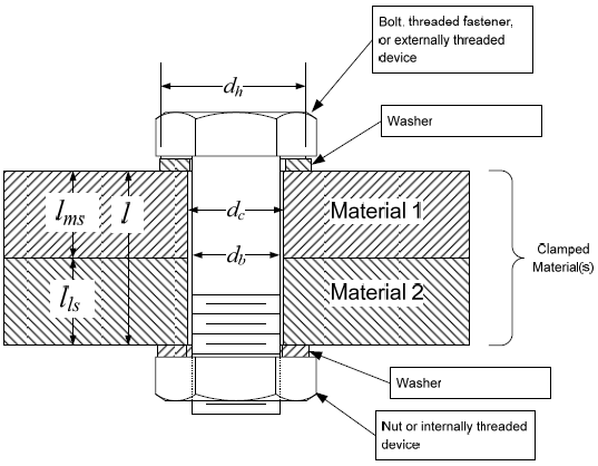
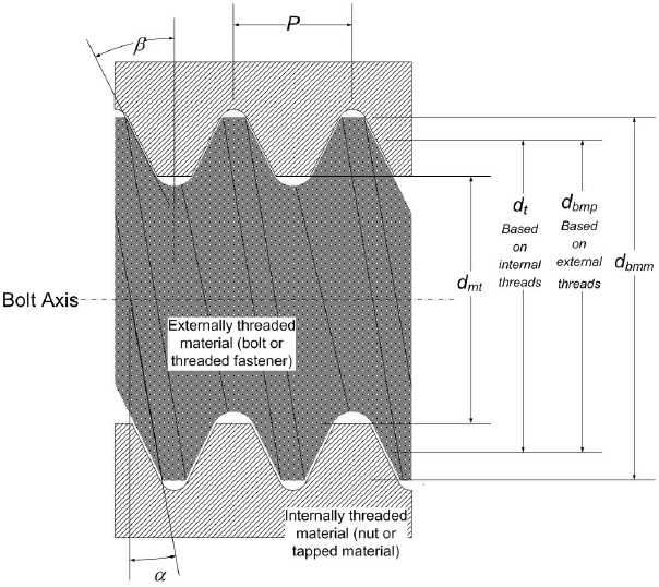
While this joint includes washers on both ends, many bolted joints do not use washers and the methodologies presented in this document apply to bolted joints with or without washers. A clearance between the bolt and the clamped materials can be accounted for, however, the methodologies presented here assume a single clearance that applies to all the layers. Figure 2 identifies important geometric parameters for a thread joint.
The guidelines NASA [11] used for bolted joints on the space shuttle are generally applicable and are adopted here.
A preloaded joint must meet, as a minimum, the following three basic requirements:
Bolt strength is checked at maximum external load and maximum preload, and joint separation is checked at maximum external load and minimum preload. To do this, a conservative estimate of the maximum and minimum preloads must be made, so that no factors of safety are required for these preloads. Safety factors need only be applied to external loads.
A critical component of designing bolted joints is not only determining the number of bolts, the size of them, and the placement of them but also determining the appropriate preload for the bolt and the torque that must be applied to achieve the desired preload. There is no one right choice for the preload or torque. Many factors need to be considered when making this determination. A basic guideline given in the Machinery's Handbook [12] is to use 75% of the proof strength (or 75% of 85% of the material yield strength if the proof strength is not known) for removable fasteners and 90% of the proof strength for permanent fasteners. Things to consider include the tension in the bolt and therefore the clamping force, fatigue concerns (higher preload is generally preferable), how much torque can easily be applied without risking damaging another part if the tool slips while applying the load, etc.
The Machinery's Handbook [12] and the NASA guide [11] give estimates for the accuracy of bolt preload based on application method. The NASA guide states these uncertainties should be used for all small fasteners (defined as those less than 3/4"). The results are summarized in Table 3.
| Method | Accuracy |
|---|---|
| Torque Wrench on Unlubricated Bolts [11] | ± 35% |
| Torque Wrench on Cad-Plated Bolts [11] | ± 30% |
| Torque Wrench on Lubricated Bolts [11] | ± 25% |
| Preload Indicating Washer [11] | ± 10% |
| Strain Gages [12] | ± 1% |
| Computer Controlled Wrench (Below Yield) [12] | ± 15% |
| Computer Controlled Wrench (Yield Sensing) [12] | ± 8% |
| Bolt Elongation [11] | ± 5% |
| Ultrasonic Sensing [11] | ± 5% |
A general relationship between applied torque, T , and the preload in the bolt, Fp , can be written in terms of the bolt diameter, d , and the "Nut Factor", K , as
T = K · db · FPTable 4 gives ranges for nut factors for a variety of materials and lubricants. The data is taken from the Standard Handbook of Machine Design [15]. Their data is based on multiple sources. As can be seen by examining the data, there can be large ranges of potential nut factors and as such, it is recommended in the Standard Handbook of Machine Design [15] to only use nut factors when approximate preload is sufficient for the design. For cases where strain gages can not be used, bolt extension can not be measured, load sensing washers can not be used, etc., there is no choice but use a nut factor. In these cases, any analysis should be done using a range of nut factors to bound the results. A low nut factor gives a higher preload and clamping force but puts the bolt closer to yield while a high nut factor gives a lower preload and clamping force but the capacity of the joint to resist external tensile loads has been reduced.
| Lubricant | Nut Factor | |
|---|---|---|
| Mean | Range | |
| Cadmium Plating | 0.194-0.246 | 0.153-0.328 |
| Zinc Plate | 0.332 | 0.262-0.398 |
| Black Oxide | 0.163-0.194 | 0.109-0.279 |
| Baked on PTFE | 0.092-0.112 | 0.064-0.142 |
| Molydisulfide Paste | 0.155 | 0.14-0.17 |
| Machine Oil | 0.21 | 0.20-0.225 |
| Carnaba Wax (5% Emulsion) | 0.148 | 0.12-0.165 |
| 60 Spindle Oil | 0.22 | 0.21-0.23 |
| As Received Steel Fasteners | 0.20 | 0.158-0.267 |
| Molydisulfide Grease | 0.137 | 0.10-0.16 |
| Phosphate and Oil | 0.19 | 0.15-0.23 |
| Plated Fasteners | 0.15 | |
| Grease, Oil, or Wax | 0.12 | |
Additional information on nut factors can be found in Bickford [4] and the Machinery's Handbook [12]. A summary of analytic approaches to compute a nut factor are given in Appendix A. At this point, the recommended method is to use a pre-computed nut factor from Table 4 until the analytic methods are better understood, compared to the known methods, and confidence is gained in the accuracy of the method. The analytic methods seem to produce artificially large nut factors (which produce very small preloads for a given torque). This is something that will be looked at in follow-on work to the initial release of this report.
All of the analytic approaches presented in this section implicitly assume an axisymmetic stress field. Any geometric or material effects that significantly violate this assumption make the approaches in this section invalid. This can include bolts very close together, bolts near a physical boundary (see section 5.4), non axisymmetric geometries, etc. If the bolted joint of interest does not meet these assumptions (and the additional assumptions of the approaches below) then it is recommended that a finite element analysis be used for the joint.
The general approach is to idealize a bolted joint into a pair of springs in parallel. One spring represents the bolt and other represents the clamped material. If an estimate can be obtained for the stiffness of the bolt (which is trivial) and the clamped material (which is difficult), then externally applied axial loads can be partitioned appropriately between the two and factors of safety can be computed to determine if the joint design is sufficient.
It is generally assumed that the clamped material can be viewed as a set of springs in series and an overall stiffness for the clamped material, km , can be computed as
where ki is the stiffness of the i th layer. The bolt stiffness, kb , can be estimated in terms of the cross sectional area of the bolt, Ab , Young's modulus for the bolt, Eb , and the length of the bolt, Lb , as
The total stiffness of the joint, kj, can be computed (by assuming two springs in parallel) as
kj = kb + kmThe remainder of this chapter is devoted to various methods of estimating the stiffness of the clamped material and comparing the various methods. It will be recommended that the FEA empirical models be used when they are applicable and to use Shigley's frustum approach for all other cases.
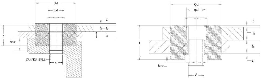
In this method it is assumed the true 'barrel shaped' stress field can be approximated as a cylinder of diameter dc (see Figure 3, dc equals Qd ). This was the original assumption made by Shigley in his first edition mechanical engineering design book [8] and is what is chosen by Bickford [4].
A factor, Q , is defined as the ratio between the actual bolt diameter and the idealized cylindrical stress field
By considering the layer as a one dimensional spring, the stiffness of the i th layer can be computed as
The area of the i th layer can be computed, assuming the inner diameter is qidb (where qi ≥ 1 and is used to allow for clearance between the clamped material and the bolt) and the outer diameter is Qdb , as
$$ A_i = < \pi \over 4 >\left[ (Q d_b)^2 - (q_i d_b)^2 \right] = < \pi \over 4 >~d_b^2 ~(Q^2 - q_i^2) $$The addition of qi is a logical extension to account for clearance holes that were included in the work of Pulling, et. al. [13] and is adopted here. The axial stiffness of the clamped material can be written as
$$ k_Pulling, et. al. [13], went on to define a bending stiffness for the clamped material using the same methodology. They assumed that the same material is loading in bending as was loaded axially. The approach is based on beam theory and as such they are assuming the ends (i.e. the edge of the assumed loaded material) are free (i.e. there is no rotation constraint posed by the material beyond that considered loaded). With these assumptions, the bending stiffness for each layer can be computed to be
The moment of inertia, I , for the i th layer can be computed as
$$ I_i = < \pi \over 64 >\left[ (Q d_b)^4 - (q_i d_b)^4 \right] $$Once again assuming each layer is represented by a spring in series, the bending stiffness of the clamped material can be computed as
$$ k_For the case of a bolted flange of a pipe with the bending applied to the neutral axis of the pipe, the actual load on the bolt will be more like an axial load and less like a bending load. There is an additional concern with this method because it is probable that the actual load on the bolt due to bending will be higher than what this theory predicts (i.e. this does not produce conservative results). This is a major concern and great care must be taken when considering bending loads on bolted joints with this method.
The original guideline put out by Pulling, et. al. [13] used a value of 3 for Q. This is the value Shigley used in the 1st edition of Mechanical Engineering Design. The accuracy of this method is highly dependent on the choice of Q. As can be seen, Q is squared (or raised to the 4th power for bending), and therefore any errors in Q are magnified. As will be shown by comparing the different methods in a later section, the value of Q is variable and depends on the geometry of the joint.
Bickford [4] noted that spheres, cylinders and frustums could all be used. He also chose to use a cylinder. He derived the same expressions for axial loading that were shown above (except he did not include qi to account for clearance) and provided the following guidance for Q (actually he provided guidance for the area of the cylinder which implies Q). His equations are modified here to account for qi so that it can be compared to the work of Pulling [13]. For the case where the bolt head diameter (or washer diameter) is greater than the joint "diameter" of the material being clamped, the entire area is used so
$$ A = < \pi \over 4 >\left[ D_J^ <~2>- (q d_b)^2 \right] = < \pi \over 4 >\left[ (Q d_b)^2 - (q d_b)^2 \right] ~~\text~~ d_h \ge D_J $$
where DJ is the diameter of the joint. This implies
$$ Q = < D_J \over d >~~\textFor the case where the joint "diameter" is greater than the diameter of the bolt head (or washer) but less than three times the diameter, the area that should be used is
The first term accounts for all the area under the bolt (or washer). The second term accounts for additional material based on the thickness, l , of the joint. This implies a Q factor of
$$ Q = <1 \over d>\sqrt < d_h^2 + \left( - 1 \right) \left( + \right) > ~~\text~~ d_h \lt D_J \le 3 d_h $$For the case where the joint "diameter" is greater than three times the diameter the of the bolt (or washer), the area that should be used is
$$ A = <\pi \over 4>\left[ \left( d_h + \right)^2 - (q d_b)^2 \right] ~~\text~~ D_J \gt 3 d_h ~~\text~~ l \le 8 d_h $$
Again it can be seen that the equation above accounts for the materials under the bolt plus additional material that is dependent on the thickness of the joint. This implies a Q factor of
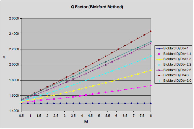
$$ Q = <1 \over d_b>\left( d_h + \right) ~~\text~~ D_J \gt 3 d_h ~~\text~~ l \le 8 d_h $$A plot of Q for various thicknesses and DJ/dh ratios is shown in Figure 4. The data was generated assuming a 5/8" diameter bolt, d , with a bolt head diameter of 15/16" (1.5 time the bolt diameter), dh . From this data we can see there is a large variation in Q depending on the thickness of the joint relative to the bolt diameter and the joint diameter (i.e. how much material is being clamped) relative to the bolt diameter.
Shigley [16] used a similar methodology but made a different assumption about the shape of the stress field to better correlate with experimental data. In this method, the stiffness in a layer is obtained by assuming the stress field looks like a frustum of a hollow cone (See Figure 5).
By assuming a 1D (i.e. axial) compression (see Shigley [16] for the complete derivation), the stiffness of a layer can be computed as
$$ k_i = < \pi ~E ~d_b \tan(\alpha) \over \ln \left(< (2 l \tan(\alpha) + d_h - d_b)(d_h + d_b) \over (2 l \tan(\alpha) + d_h + d_b)(d_h - d_b) >\right) > $$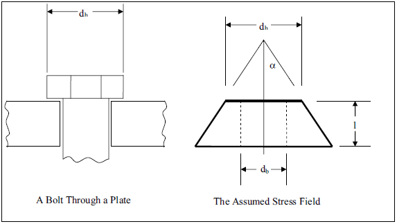
Various angles, α , have been used. 45 degrees is often used but this often over estimates the clamping stiffness. Shigley states that typically the angle to use should be between 25 and 33 degrees and in general recommends 30 degrees (this is assuming a washer is used). There are two obvious examples when this falls apart. The first is for the case when there is not enough material for the frustum to exist (e.g., a bolt hole very near an edge of a plate). The second case is for very thick clamping areas. For this case, the shape of the actual stress distribution looks more like a barrel and the shape assumed by Shigley is inappropriate.
There are a number of subtleties that must be noted based on the assumptions in this method. First, there must be 'symmetric' frustums across the entire joint regardless of the number of materials (otherwise static equilibrium would not be met). The value of D used for a given layer must take into account the frustum of the previous layer and not just the bolt or washer diameter. The actual value of dh that really should be used is the start of the stress frustum and not the diameter of the bolt head and/or washer. Due to flexibility in the bolt or washer, the correct value of dh will be less than the bolt head (or washer) diameter and the degree to which it is less depends on the relative stiffness of the materials involved. If the bolt is in a threaded hole, the starting point for the frustum at the threaded end should be at the bolt threads and this is typically assumed to be at the midpoint of the engaged threads and dh is typically used instead of db . This is not strictly correct but is accurate enough with all the other assumptions built into the method. The actual point of where one frustum begins and the other ends must be computed for each layer.
It should be pointed out that Shigley [16] suggests that the work of Wileman [17] is the preferred method (when it is applicable) to the frustum approach presented here. It, and extensions to it, will be presented in the next section. It is assumed by the authors that this is because it is a simpler method not because it is necessarily more accurate. As will be shown, the results for the frustum approach and the Wileman approach produce very similar results for joints with only one material.
Wileman [17] used finite element analysis to determine the clamped material stiffness for two "plates" made of the same material. It is based on a standard spring stiffness model for the overall joint that was previously discussed. The results of this work produce a clamped material stiffness for commercial metals of
$$ k_m = 0.78952 ~E ~d_b ~e^ < 0.62914 ~d_b / l >$$where E is the Young's modulus of the material, db is the diameter of the bolt and l is the thickness of the clamped materials (i.e. the two "plates").
Musto [10] extended this approach to two materials by introducing two new variables
$$ E_where ms denotes the 'more stiff' material and ls denotes the 'less stiff' material. He then proposed the clamped material stiffness to be
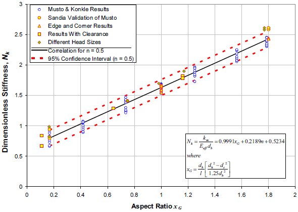
$$ k_m = E_and computed valued of m and b based on different materials stiffness ratios between materials and ratios of bolt diameter to clamped material length. Durbin, Morrow, and Petti [9] analyzed Musto's results and concluded a general purpose equation across materials and geometries could be written. They also extended the work to address clearances, edge effects and variable bolt head diameters. They determined the clamped material stiffness including accounting for clearances, edge effects and variable bolt head diameters can be written as
$$ k_m = E_This relationship is valid for aspect ratios of bolt diameter to length of clamped material between 0.167 and 1.786, and is still restricted to two materials. The correlation has a standard error of 0.065. Figure 6 shows the correlation and how it matches to the finite element data.
Durbin et al. [9] compared this equation to the one derived for the Q-factor method and noted the only unknown between the two equations is Q . They implemented an iterative solve for Q and incorporated that into an updated spreadsheet based on the original work of Pulling [13].
Durbin, Morrow and Petti [6] examined boundary effects of bolted joints when the bolt head diameter (or washer) is 1.5 times larger than the bolt diameter and in the restricted db/l range of 0.167 to 1.786. They followed the methodology of Musto [10] that was described in the previous section and looked at both edge effects and corner effects. They concluded that there is not significant degradation of the joint until the edge or corner effect is within 1.5 bolt diameters of the hole. As such, the methods described in the previous section should be applicable to most bolted joints.
To get a quantitative comparison of the various analytic method relative to one another, consider the case of 5/8" bolt with a bolt head diameter of 15/16" (1.5 times the bolt diameter) clamping two "plates" of the same material. In this case, it is possible to solve for an equivalent Q for each method. We will only consider cases where there is significant clamped materials around the bolt (i.e. the surrounding joint contains material to at least three times the bolt diameter). This data is shown in Figure 7.
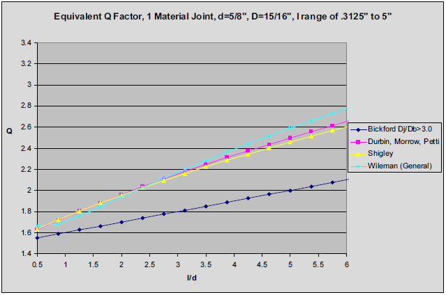
As expected, the Wileman [17] and Morrow [9] methods produce similar results since Morrow's fit is based on extensions to Wileman's work. The differences are likely due to the fact that Morrow's data covers multiple materials in addition to various geometries and Wilemans's data is for a single material. Shigley's method [16] is also similar to the other two methods. The divergence in the methods occurs as the clamped material gets thick compared to the bolt diameter. Bickford's [4] method is dramatically different than the other 2 and in comparison will produce much lower clamped material stiffness. It appears it is overly conservative and will not be considered further in this document.
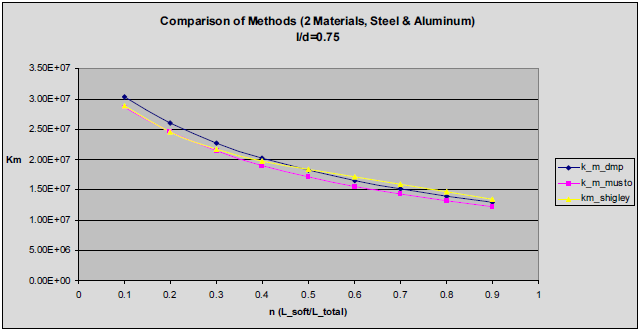
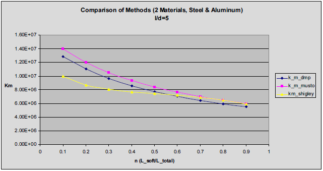
The next comparison that can be made is using two materials for Shigley's method [16] and the extension of Wileman [17] by Musto [10] and then Morrow [9]. Again consider the case of 5/8" bolt with a bolt head diameter of 15/16" (1.5 times the bolt diameter) clamping two "plates". In this case, one "plate" will be made from steel and the other plate from aluminum. The relative amount of each material will be varied from 10% to 90% of the total joint thickness. Figure 8 shows the results for an l/db ratio of 0.75 (this represents a "thin" clamped joint) and Figure 9 shows the results for an l/db ratio of 5.0 (this represents a "thick" clamped joint). As can be seen in Figure 8 the methods produce very similar results for "thin" clamped joints. As can be seen in Figure 9, the methods are very similar for "thick" clamped joints when there is a significant fraction of soft material (i.e. aluminum in this case), but significant differences when there is a significant fraction of stiff material (i.e. steel in this case). Although not shown, this significant difference begins at roughly an l/db ratio of about 2.0.
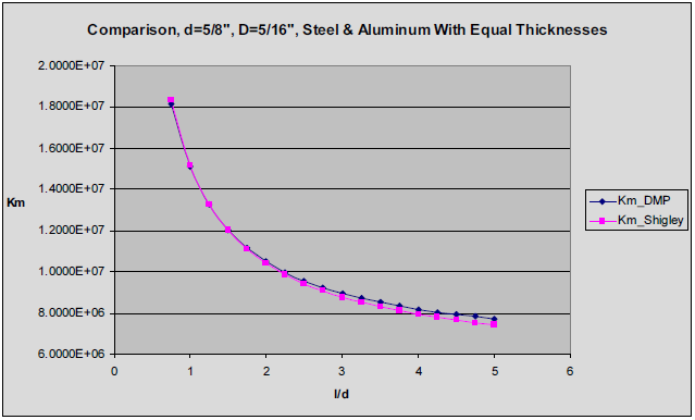
In Figure 9 it can be noted that the results look similar for equal thicknesses of the two materials (i.e. at n = 0.5 ) at the bounds. Figure 10 shows the results for n = 0.5 across the range of l/d ratios. The methods produce very similar results. The trends of Morrow [9] seem to be more physically intuitive and are backed up by finite element analysis. The Shigley method must use 3 frustums for n ≠ 0.5 because the 'knee' is not at the interface. The use of 3 frustums introduces some error as discussed previously. Based on this, it is recommended to use the Morrow method whenever only 2 layers of material are being clamped and the l/db ratio is within their recommended bounds. Otherwise, the Shigley method is recommended. A follow on to this work will be to extend the Morrow method to more than two materials and verify the results.
All of the analytic or empirical approaches presented in this chapter make assumptions and are quite good in many cases but none applies in every case. Nonetheless, these methods constitute the first tool available to an engineer looking at bolted joints. In general, it is recommended to use these types of approaches and evaluate if a higher fidelity analysis is required.
In summary, three approaches to calculating joint stiffness have been presented. The first is a method based on an assumed cylindrical stress field. Bickford's [4] and Pulling's [13] work is based on this assumption. The positives of this method include the overall simplicity of the application of the method, the simplicity with which the effect of clearance holes can be accounted for, and that an extension to including bending to the factor of safety calculations may be included (although they should be used with great care since the underlying assumptions are based on beam theory accurately portraying the joint). The down side of this method is that the accuracy is highly dependent on the choice of Q (or the area). The axial stiffness computed by this method is proportional to Q 2 and the bending stiffness computed by this method is proportional to Q 4 . As such, small errors in Q become large errors in the member stiffness. The data shown in Figure 7 indicates that Q can reasonably vary from 1.6 to 2.6 depending on the geometry. The second method, from Shigley [16], is based on an assumption the stress field can be represented as a hollow frustum of a cone. While there are subtleties to applying the method, it has been used successfully since the 1960's for designing and analyzing bolted joints and it is general enough to apply to any axisymmetric geometry (although the accuracy is unknown at best or questionable at worst for anything but simple geometries). The third method is based on using finite element analysis of bolted joints and fitting the results with empirical equations. The work of Wileman [17], Musto [10] and Morrow [9] are all based on this method and each is an extension of the previous work. In the latest form, this method has been shown to be applicable to most commercial metals (including Steel, Aluminum, Brass and Titanium) and a wide range of geometries including two-material joints. The method is the easiest to apply and has been 'verified' since it was based on finite element calculations. The down side is that it is only applicable for two layer joints and only applies in certain ranges of geometries (although it should be noted the range is relatively broad and likely to cover most engineering applications).
The ultimate choice is of course left up to the engineer designing and/or analyzing the joint. Any of the methods can be used successfully if the engineer is aware of the assumptions and limitations and applies the theory correctly. Based on the pros and cons of each method, it is recommended that the empirical method of Morrow [9] be used as the preferred method when it is applicable. In cases, where it is not, it is recommended that the hollow frustum approach of Shigley [16] be used. The reasons for recommending the DMP method are 1) it matches very well with finite element analysis and Shigley's frustum approach for standard cases, 2) it doesn't have the subtleties and the unknown accuracy for differing materials with different thickness (but matches extremely well for identical thicknesses where Shigley is known to be accurate) and 3) it is the easiest to apply and gives the same results in cases where both are equally applicable. It is planned for follow on work to extend the work of Morrow [9] to cases of more than two materials and perhaps to expand the range of geometries that it is applicable to. For cases where a high degree of accuracy is required, the geometries and/or materials don't match the assumptions of these analytic methods, the loading is complicated, or the margins are very small, it is recommend that a finite element analysis be performed on the joint.
Now that an estimate for the bolt stiffness, kb , and the clamped material stiffness, km , has been obtained, we can examine how an externally applied tensile load is partitioned between them. An applied axial load, F , will produce a displacement, δ . Part of the load will be taken up by the bolt, Fb , and part will be taken up by the clamped material, Fm . We know the bolt and the clamped material act as springs in parallel so we can solve for the total displacement (assuming the joint is not loaded to the point where the material is no longer clamped which is complete failure of the joint) as
The stiffness constant, C , of the joint is defined to be the ratio of the load taken by the bolt to that of the joint as a whole and can be computed as